MS Excel formula question

wheelsup_cavu · July 14, 2021, 10:41pm

Hello Mudpikers,

Looking for some MS Excel help.

I am able to create a nested “IF” formula to search a prior cell for a specific condition but I want a formula or a Conditional Formatting option that searches for a specific condition until it finds that condition in any previous cell when the prior cell does not generate the correct condition. Gas in column B is what I want the formula to find.

Here is a page from the Excel chart I created for my vehicles service records.

My problem is when I get two cells in a row that generate a Service condition the MPG results are incorrect because the “IF” condition I created only jumps back one cell for the Mileage. What I need is a formula that jumps back to the first prior Gas condition.

I am aware that I could combine the Information in Cells 294 and 295 which would make my formula function correctly but I am trying to keep the information Date correct.

My current IF formula for Row 295.

=IF(D295="","Service",IF(E294="Service",(C295-C293)/D295,(C295-C294)/D295))

The problem with this formula is caused in row 296 of this chart because there are two cells in a row that create the “Service” Condition.

=IF(D296="","Service",IF(E295="Service",(C296-C294)/D296,(C296-C295)/D296))

I do not want to create a separate formula for each condition, or a nested IF condition that still will not solve for every situation, so I am hoping there is a Conditional formatting option that will solve my problem.

Wheels

Rhinosaurus · July 15, 2021, 1:01am

I could probably solve this fairly quickly if I was at home

I think invoking isnumber in the if statement would help but do this on my phone is not optimal.

Rhinosaurus · July 15, 2021, 2:02am

Can you email me the file? Or link me via Google? I can see what going on in sheets.

I’m not an expert but I mess with excel on an intermediate+ basis daily.

wheelsup_cavu · July 15, 2021, 5:33pm

Here is the file @Rhinosaurus . Thanks for the help.
vehicle_maintenanace_logs.zip (6.4 KB)

Wheels

Rhinosaurus · July 15, 2021, 5:52pm

Will have access to a computer this evening so I’ll take a look then.

keets · July 15, 2021, 10:45pm

Rather than do the next row formula thing in your data table, couldn’t you have a raw data table/tab and then use a separate tab with a new table and lookup formula in the if statement to pull out the values from the master table? #thatmakesmoresensetomewheniwroteit

If I get time I’ll have a look tomorrow, with @Rhinosaurus looking at it as well, hopefully you’ll get a quick solution.

jenrick · July 16, 2021, 12:12am

So I’m clear on how you want to do this, you want to take the amount of gas added in column D, and using the mileage difference calucated from column C figure out the MPG in column E.

So for say E304, it’s (C304-C303)/D304 Do I have that right?

Rhinosaurus · July 16, 2021, 1:46am

I’m not sure if I’m just too tired or what but I am not getting this to work. Interested to see what others come up with.

wheelsup_cavu · July 16, 2021, 2:22am

I am open to any ideas @keets . I am a novice when it comes to using Excel and entirely self taught so my choices are likely to be some of the least efficient.

That is the correct formula for those cells @jenrick.
If all I was doing with the chart was calculating the gas mileage the formula would be a simple one like you show but once I throw the service records into the chart I create my problem. For row 296 I need a formula that jumps to row 293 since that is the prior Gas entry.

E296, it’s (C296-C293)/D296

Have a few hours into this math teaser myself so I understand.

Thanks for the help everyone.

Wheels

keets · July 16, 2021, 8:32am

Try this… @wheelsup_cavu

vehicle_maintenanace_logs.zip (10.2 KB)

What I’ve done is create an extra column, mileage at last fill up, which returns the last mileage when Gas was in column B.

jenrick · July 16, 2021, 10:49pm

Try this

So in short we have a couple things we need to do:

1)Figure out if we we need to even run the MPG calculation, your first IF statement does this just fine.

2)Next if we do need to run the MPG calculation we need to find the previous mileage to use. To do this we need to find the most recent valid gallons of gas entry. LOOKUP will sort through a column/row/array looking for a value and then return it when it finds it. What we want is when it doesn’t find it. It will respond with the last valid entry. So in this case we tell it to look for an gas value of 1000, which it obviously won’t find. So it will go to the end of the list of entries and take the last value. All we need to do is set it so it only searches the list of all gas values BEFORE the current record. So if we are on record 19, we only want it to check records 1-18, and so on. It doesn’t count blanks so it simply skips them back up to the last row with a valid numerical entry, thus handling the multiple service entries.

So far we have (assuming we are on record 19) =LOOKUP(1000,D$1:D18) This will return the last gas value in column B for row 1-18, which should give us our most recent fill up record.

Now returning the gas value itself doesn’t do much for us, but we can tell the formula to instead return the value in another part of the worksheet that has the same row/column as the set we’re searching. We need the mileage in column C, so our formula now reads =LOOKUP(1000,D$1:D18,C$1:C18). This will return the mileage value in the corresponding cell in column C.

Now you may note the $ before the cell number, this is to force excel to not try and get smart about updating that reference when copying and pasting, or filling. If I fill down 10 cells to record 29, excel will update the formula, but wont change the items that have the $ symbol. So the formula in record 29 is =LOOKUP(1000,D$1:D29,C$1:C29) automatically without having to go in an update the formula.

C) The last step is to simply do the math to determine MPG.

So the whole formula looks like this:

=IF(D34=“”,“Service”,((C34-(lookup(10000,D$11:D33,C$11:C33)))/D34))

It works in sheets, so let me know if it doesn’t run in excel. To extend the records down, either copy and past it into the next record, or just fill down as needed.

Rhinosaurus · July 16, 2021, 11:07pm

I wonder what I had wrong here because that’s essentially what I was doing (not using 1000 but same formula) and I kept getting an error.

jenrick · July 17, 2021, 12:37am

Depending on how you had the lookup referenced, column or array it can get picky.

keets · July 17, 2021, 1:19am

The file I posted up there has the solution working in a similar way @jenrick.

wheelsup_cavu · July 17, 2021, 5:27am

Thanks for the ideas.
Will have to work with them later Saturday, going to Burbank airport first thing Saturday morning, or Sunday.

Wheels

wheelsup_cavu · October 15, 2021, 5:50pm

Excel file:
blood_pressure-mudspike.zip (10.7 KB)

I have another Excel formula question that maybe we can resolve? I am trying to get a cell to automatically reference another cell when the value changes. What I want is for the date in column A to be placed in Cells D5 and D6 when then information in columns F and G match the information in Cells B5 and/or B6 and C5 and/or C6.

This formula is not working the way I want but it is doing something that is close.

(Cell D5) =IF((MAX(G:G))=B5,(A:A),"Nope")

(Cell D6) =IF((MIN(G:G))=B6,(A:A),"Nope")

As you can see in the image the formula I am using is pulling the information from Column A, Highest BMI and Lowest BMI, instead of “Nope” so it is working but not the way I want. In cell D5 where it is showing “HIghest BMI” in the cell it should be placing the information from cell A13, March 16, 2021, in that cell if the formula was working the way I wanted. The information I want in Cell D6 is not shown in the image but in the Excel file I attached it should be pulling the information from cell A47, October 10, 2021.

Wheels

keets · October 16, 2021, 7:22am

As a starting point, you need to look at learning how VLOOKUP works. It helps you solve so many things in excel when you have a bunch of data you need to return based upon another piece of data in a different column.

Put simply, VLOOKUP allows you to scan a table of data for a value, then pull other data in that row.

Your table of data in the image you’ve provided as an example this case is A9:G31. The number for column G will be the last row you have in the data.

You’ll need to play about with a nested IF statement in the VLOOKUP to check the range of the BMI and weight for the conditions, but then the VLOOKUP pulls the first column when it’s what you want.

I might get chance later to download your file later, if you’re struggling.

wheelsup_cavu · October 16, 2021, 1:49pm

Edit:
I believe I solved my riddle by using the Index/Match functions in a nested formula. Will do some more testing this afternoon after I get back from my errands. If my fix continues to work properly I will upload the working spreadsheet and leave a link to the website’s tutorial.

I did some searching online last night and the Vlookup function looked the most promising. I did not understand how it worked even after looking at the examples I found online last night. Will give ye olde online search another go today but any help will be appreciated.

Wheels

wheelsup_cavu · October 16, 2021, 10:12pm

Excel file with INDEX/MATCH fix. blood_pressure-mudspike-01.zip (10.7 KB)

This fix was a strictly monkey see monkey do copy and paste affair for the most part. I do not fully understand why it is working I just know that it is working. When I used the VLOOKUP function in my spreadsheet I kept getting the #N/A error message. When I searched for a way to resolve that error I found the INDEX/MATCH solution.

Here is a link to the webpage where I found the example I used in the Excel spreadsheet I uploaded to this post.

How to correct a #N/A error in the VLOOKUP function: How to correct a #N/A error in the VLOOKUP function - Microsoft Support

Consider using INDEX/MATCH instead

INDEX and MATCH are good options for many cases in which VLOOKUP does not meet your needs. The key advantage of INDEX/MATCH is that you can look up a value in a column in any location in the lookup table. INDEX returns a value from a specified table/range—according to its position. MATCH returns the relative position of a value in a table/range. Use INDEX and MATCH together in a formula to look up a value in a table/array by specifying the relative position of the value in the table/array.

Syntax

To build syntax for INDEX/MATCH, you need to use the array/reference argument from the INDEX function and nest the MATCH syntax inside of it. This take the form:

=INDEX(array or reference, MATCH(lookup_value,lookup_array,[match_type])

Let’s use INDEX/MATCH to replace VLOOKUP from the example above. The syntax will look like this:

=INDEX(C2:C10,MATCH(B13,B2:B10,0))
In simple English it means:

=INDEX(return a value from C2:C10, that will MATCH(Kale, which is somewhere in the B2:B10 array, in which the return value is the first value corresponding to Kale))

****(If you look at the image from their example you will see that they have placed an extra comma 0 in the formula. =INDEX(C2:C10,MATCH(B13,B2:B10,0),0) The formula works with or without that extra comma 0 but I put it in because they show it in their image example. I have no clue what it does, yet.)

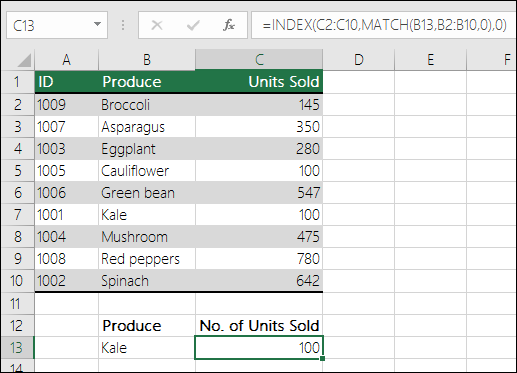
The formula looks for the first value in C2:C10 that corresponds to Kale (in B7) and returns the value in C7 ( 100 ), which is the first value that matches Kale.

Here are my formulas I created from that tutorial page.

Cell D5: =INDEX(A9:A25000,MATCH(B5,G9:G25000,0),0)
=INDEX(return a value from A9:A25000, that will MATCH(Cell B5, which is somewhere in the G9:G25000 array, in which the return value is the first value corresponding to B5),0)

Cell D6: =INDEX(A9:A25000,MATCH(B6,G9:G25000,0),0)

This image shows that the formulas are returning the correct information from my spreadsheet in cells D5 and D6.

This image shows the the Highest BMI date in cell D5 is dynamic because it changed when I changed the data cell F9.

This image shows the the Highest BMI date in cell D5 and the Lowest BMI date in cell D6 are dynamic because both cells D5 and D6 changed when I changed the data in cell F9.

Now the really pleasing part of this is that I have another spreadsheet where I thought using this INDEX/MATCH solution would be the cats meow BUT when I use it in that spreadsheet I am getting the #N/A error message once again. Lol one step forward two steps back.

Wheels

jenrick · October 17, 2021, 12:46am

Can you paste in your vlookup expression?

What gets people 99% of the time is that the first column in the data you are looking through HAS to be the column you are looking through. It will throwa N/A if doesn’t find the value so you need a catch condition for that as well.